
「自然言語処理ってなに?」「何から始めればいい?」といったお悩みを解決できるかもしれない記事になっています。 自然言語処理に対して無知すぎた自分が、BERTを学ぶ前に、まず基本的な手法の一種であるトピックモデルを学び、使えるようになりたいと思い、まとめたことを解説します。
※この記事を読む前に、以下のその1,2に目を通していただけると、この記事のテーマをよりご理解いただけると思います。
★その1

★その2

前回までの流れ
前回、文章のベクトル表現やトピックモデルまで行った。今回は、ベクトル表現やトピックモデルを実際のデータセットに用いてみる。


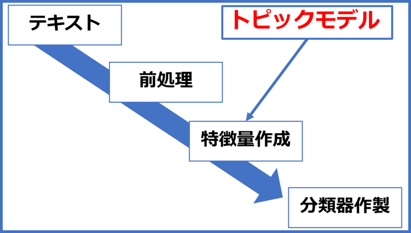
分類までの流れ
前処理→トピックモデル→分類
前処理
前記事に書きました。
特徴量作成
文章のベクトル表現やトピックモデルに関して、前記事に書きました。
実際のデータセットに用いてみる
データセット
今回はデータセットとして、IMDB映画レビューのデータセットを使ってみる。
レビューとネガポジが対になっているデータセットになっている。
詳細のドキュメントは以下のサイトにあります。
データセットの取得とデータフレーム化する。(データをよくcsvからデータフレームにすることが多いため、あとで転用できるようにするため。)
#データセットの取得
from tensorflow.keras.datasets import imdb
# imdb = imdb
(train_data, train_labels), (test_data, test_labels) = imdb.load_data()
#数値で取得しているため、テキストデータに戻す。
word_index = imdb.get_word_index()
# 最初の要素を予約(単語を登録)
word_index = {k:(v+3) for k,v in word_index.items()}
word_index["<PAD>"] = 0
word_index["<START>"] = 1
word_index["<UNK>"] = 2
word_index["<UNUSED>"] = 3
reverse_word_index = dict([(value, key) for (key, value) in word_index.items()])
def decode_review(text):
return ' '.join([reverse_word_index.get(i, '?') for i in text])
#データをDataFrameにする。(csvとかで取得した際、to_csvでDFにすることが多いため)
import pandas as pd
train_df=pd.DataFrame(train_data)[0].map(decode_review)[::5].reset_index(drop=True)#データを軽くするため
test_df=pd.DataFrame(test_data)[0].map(decode_review)
DataFrameのデータに対して前処理
clean_text_df=train_df.map(clean_text)
clean_text_df
1つ目の文章の一部を見てみる。
“
↓
‘film brilliant cast location scenery story direction everyone really suit part play could imagine robert redford amaze actor director norman father come scottish island love fact real connection film witty remark throughout film great brilliant ….
いらない箇所が除去され、文章が簡略化されている。
こんな感じで前処理を行い、そして文字を区切って準備完了。
input_dataset=clean_text_df.values
texts = [
    [w for w in doc.lower().split() if w not in stopwords.words('english')]
        for doc in input_dataset
]
実際にこのデータでLSI,LDAモデルを作成し、どんなことができるか考えてみる。
BoWでLSI、LDAの学習
まずは、コーパス作製する。
import collections
import gensim
dictionary = gensim.corpora.Dictionary(texts)
corpus = [dictionary.doc2bow(text) for text in texts]
#一部の分析には不必要な単語を除去するための以下
count = collections.Counter(w for doc in texts for w in doc)
tokens_num = len(count.most_common())
N = int(tokens_num *0.01)
max_freq = count.most_common()[N][1]
#出現回数が上位1%以上や5回以下の単語を除去
corpus = [[w for w in doc if max_freq > w[1] >= 5] for doc in corpus]
学習する。
num_topics = 8
lsi = gensim.models.LsiModel(
corpus=corpus,
num_topics=num_topics,
id2word=dictionary,
random_seed=42
)
num_topics = 8
lda = gensim.models.ldamodel.LdaModel(
corpus=corpus,
num_topics=num_topics,
id2word=dictionary,
random_state=42
)
予測した中身を確認してみる。
#BoWでlda,lsiモデルで予測の学習からwordcloudの作製
test_text=test_df[0]
print(test_text)
text = clean_text(test_text)
text = dictionary.doc2bow(text.split())
lsi[text],lda[text]
LSI結果
[(0, 0.2441218427800891),
(1, 0.1489563371647855),
(2, 1.930518715934596),
(3, 0.7241376257978716),
(4, 0.6893975568334086),
(5, -0.7141122152541468),
(6, 0.08167571315801359),
(7, -0.12309210947077602)]
LDA結果
[(0, 0.19003183),
(1, 0.28995863),
(4, 0.22779427),
(5, 0.12999244),
(6, 0.09702844),
(7, 0.054603953)]
このような感じでトピック予測ができた。
実際に計算結果からwordcloudを作製してみた。(左2列LSI、右2列LDA)


トピック毎、モデルごとに異なった特徴をつかんでいる。
tfidfでLSI、LDAの学習からwordcloudの作製
まずは、コーパス作製する。
dictionary = gensim.corpora.Dictionary(texts)
corpus = [dictionary.doc2bow(text) for text in texts]
tfidf = gensim.models.TfidfModel(corpus)
corpus_tfidf=tfidf[corpus]
学習する。
num_topics = 8
lda_tfidf=gensim.models.ldamodel.LdaModel(
corpus=corpus_tfidf,
num_topics=num_topics,
id2word=dictionary,
random_state=42
)
num_topics = 8
lsi_tfidf=gensim.models.lsimodel.LsiModel(
corpus=corpus_tfidf,
num_topics=num_topics,
id2word=dictionary,
random_seed=42
)
#lda,lsiモデルで予測
test_text=test_df[0]
print(test_text)
test_text_ = clean_text(test_text)
test_text_ = dictionary.doc2bow(test_text_.split())
text_tfidf=tfidf[test_text_]
# lsi_tfidf[text_tfidf],lsi_tfidf[text_tfidf]
lsi_tfidf[text_tfidf],lda_tfidf[text_tfidf]lsiの結果
[(0, 0.08883806350680234),
(1, -0.007826572220074544),
(2, 0.015469974534216656),
(3, -0.0069660072323797645),
(4, 0.021359336595368834),
(5, -0.03414896801062161),
(6, 0.008812985189922346),
(7, -0.0002751536784505176)]
ldaの結果
[(0, 0.6480108),
(1, 0.028845962),
(2, 0.028843114),
(3, 0.17838849),
(4, 0.028869865),
(5, 0.028840661),
(6, 0.02884181),
(7, 0.029359294)]
実際に計算結果からwordcloudを作製してみた。(左2列LSI_tfidf、右2列LDA_tfidf)


こっちの場合もトピック毎、モデルごとに異なった特徴をつかんでいる。
まとめ
次回
分類器を用いて学習・分類予測までを行う。
その4のリンクです。
もし、この記事を読んで参考になった・他の記事も読んでみたいと思った方、twitterのフォローボタンを押していただけるとモチベーション向上につながるので、よろしくお願いいたします。
ChatGPTについて
大規模言語モデル等の台頭により、トピックモデルはなかなか学ばなくなってしまった気もしますので、最近学んだChatGPTでどういう文章を送ればよい答えが返ってくるかということをまとめてみました。

コメント